Backpropagation is the cornerstone of the deep learning paradigm – the idea that learning is nothing more than optimizing some composition of differentiable functions. In fact, it is the very algorithm that allows neural nets to learn! But it is really only one of the many applications of an even broader numerical computing technique known as automatic differentiation.

Automatic differentiation's contribution to neural nets is perhaps its most popularized use today, but the idea has a long history, and its story is ongoing. While our discussion of the technique will be phrased in terms of its utility to neural nets, the lessons gleaned from studying it are far more applicable, illustrating some deeper truths about differentiation, dynamic programming, and the art of problem solving in general.

What follows is a concise review of multivariable calculus, before we delve into some more complex math. Regardless of your skill level, it may help to codify (or at least revisit) the basic intuitions behind the classical conception of the derivative, because we will need these foundations to build up to some more involved ideas. Of course, if you'd like to get right into things, you're welcome skip ahead. That said, let's begin!

Learning to Differentiate

Derivatives of single-variable functions are measurements of how infinitesimal variations to a function's input-space correspond to the resulting variations in its output-space. And the same is true of multivariable functions, except now we have many more ways in which to vary our input-space.

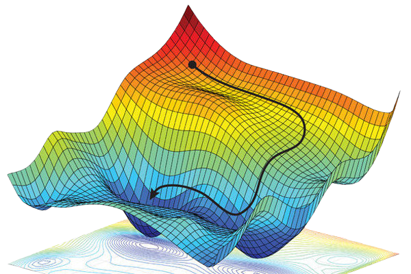
To start, let’s consider a function of two variables. Such a function can be pictured as a surface above the Cartesian plane, where the height of a point on that surface is calculated using the function \(f(x,y)\) in question. With this in mind, the geometrical interpretation of the derivative is how the elevation of this surface changes given a small step in some direction.

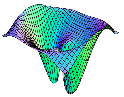
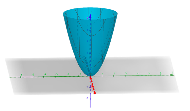
An important thing to notice here is that this step could be in any direction: the \(x\) direction, \(y\) direction, or some combination of the two. Say, for instance, we wanted to differentiate the function \(f(x,y) = x^2 +y^2\) with respect to \(x\). We now know what this means geometrically, but how exactly would we go about calculating it?

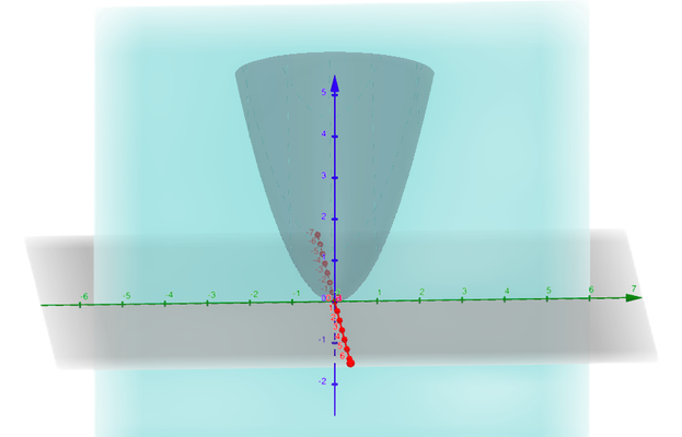
Imagine standing at some point on this function's surface, and walking horizontally in both directions. If we walk such that a spool of yarn unravels behind us, the shape this yarn takes will resemble the graph of the single-variate function \(f(x) = x^2 +C\) (a parabola) where \(C\) is some constant, namely whatever the \(y\)-value of our original point was.

It's not immediately obvious, but by walking horizontally across our surface we only varied our \(x\)-coordinate, while our \(y\)-coordinate remained constant. When walking in this way, the surface is described by a special case of the original function where \(y\) is a constant.

Similarly, a walk in a purely vertical direction is described when \(x\) is a constant. In fact, we would find that all multivariable functions behave in this way when being walked upon in the direction of one of their variables, such that all others become constants.

In that vein of thought, we might conjecture that when computing the derivative of our function \(f(x,y) = x^2 + y^2\) with respect to \(x\), we can imagine we are instead differentiating \(f(x) = x^2+C\), as this is what the surface looks like when moving in the \(x\) direction. Then the derivative with respect to \(x\) (what we call the partial derivative) would be \(2x\), or \(\frac{\partial f}{\partial x} = 2x\).

And it turns out that this thought is in fact correct!¹ When taking the derivative of a multivariable function with respect to only a single variable, we can treat all other variables as constants and just apply our single-variable differentiation rules.

But how do we generalize this idea when taking steps across our surface that aren't only in the \(x\) direction or only in the \(y\) direction, but rather some combination of both? For instance, how would we calculate the derivative for some infinitesimal step along the vector \(\langle1,1\rangle\)?

Well, a step in this direction is equivalent to one step in both the \(x\) direction and \(y\) direction. And since we know how our function changes for a pure step in the \(x\) direction \((\frac{\partial f}{\partial x} = 2x)\) and \(y\) direction \((\frac{\partial f}{\partial y} = 2y)\), the derivative in this direction is just their sum: \(\frac{\partial f}{\partial x} + \frac{\partial f}{\partial y} = 2x + 2y\).

More generally, given any vector \(\boldsymbol{\vec{v}}\), we can compute its corresponding derivative – or directional derivative – by dotting it with the vector containing our function's partials.

\(D_\boldsymbol{\vec{v}}f(x_1, x_2, \ldots, x_n) = \boldsymbol{\vec{v}} \cdot \begin{bmatrix} \frac{\partial f}{\partial x_1}\\ \frac{\partial f}{\partial x_2}\\ \vdots \\ \frac{\partial f}{\partial x_n}\\ \end{bmatrix}\)

We can now calculate all of a function's possible derivatives. A natural question then, is what derivative is the greatest? In what direction does a function increase most rapidly?

The equation for directional derivatives says that the derivative with respect to some vector is that vector dotted with the vector of our function's partials, so answering this question means finding whatever vector yields the largest possible dot product in this situation.

And since a vector's dot product is largest when dotted against itself, the vector that maximizes this dot product is the vector containing all the partials of our function! So the direction represented by this vector must be the direction of steepest ascent – the greatest derivative of our function.

Intuitively, this makes sense too, as how much this vector points in a given direction is equivalent to the derivative in that direction, such that it points more in steeper directions and less in shallow ones, thus becoming the steepest direction itself. This vector is known as a function's gradient, and is denoted like so:

$$\nabla(x_1, x_2, \ldots, x_n) = \begin{bmatrix} \frac{\partial f}{\partial x_1}\\ \frac{\partial f}{\partial x_2}\\ \vdots \\ \frac{\partial f}{\partial x_n}\\ \end{bmatrix}$$

Gradient Descent

With this bit of multivariable calculus under our belt, we can now bring neural nets into the picture. As a quick review, we think of neural nets as universal function approximators. If given enough data and made deep enough, they can represent any conceivable function.

And what gives them this ability is their constituent unit, the neuron: a computational machine with the ability to learn. Mathematically, a neuron's activation (output) is defined like so, where \(\boldsymbol{\vec{x}}\) is some input vector, \(\boldsymbol{\vec{w}}\) and \(b\) are the neuron's two learnable parameters (known as a weight and bias, respectively) and \(\sigma\) denotes some non-linearity:

$$\alpha = \sigma(\boldsymbol{\vec{x}} \cdot \boldsymbol{\vec{w}} + b)$$

We refer to a neuron's parameters as learnable because they can be updated such that the neuron returns the desired output for a given input. And somewhat counter to intuition, by stacking these simplistic units together, we can get the resulting structure – known as a neural net – to exhibit surprisingly intelligent behavior.

What's more, all of these behaviors can be framed as some sort of prediction task: given lots of labeled data, how do we optimize the parameters of all neurons in a given network such that it predicts the correct label for a given input?

All optimization is just a matter of searching the space of possibilities. If we consider only a single neuron, then this space is defined by all \((\boldsymbol{\vec{w}}, \boldsymbol{b})\) pairs that the neuron could have. But to search this space intelligently, we need to mathematically define what exactly makes a specific pair good. This means asking the question: what criterion does a good pair minimize?

Good pairs allow the neuron to make predictions that are close to the corresponding label. Said another way, they minimize the margin of error between the prediction and the correct label. If we define an error function² \(E(\hat{y}, y)\) that takes a prediction \(\hat{y}\) and and a label \(y\) and computes this margin of error, then a good pair minimizes the following objective function:

$$J(\boldsymbol{\vec{x}}, y; \boldsymbol{\theta}) = E(\alpha, y)$$

This function takes in some labeled datapoint \((\boldsymbol{\vec{x}}, y)\) and our neuron's parameters \(\boldsymbol{\theta}\). Using these, it computes our neuron's activation \(\alpha\), and passes it and the label \(y\) to our error function. It returns low values for good parameters, because good parameters generate good predictions, and good predictions have a low margin of error.

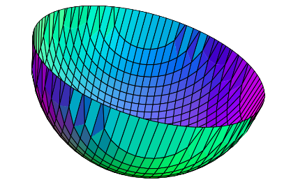
So optimizing our neuron boils down to finding parameters nestled in the local minima of this function: the valleys of whatever high-dimensional error-surface it encodes.

For a single neuron, it would be easy enough to obtain these analytically (by solving for critical points), but as we scale things up this approach quickly becomes intractable. We might instead consider the simpler sub-problem of how to get a slightly better parameter pair (instead of an optimal one), and then repeat this process over and over.

A better pair is just one for whom the function returns a lower value – so any pair on our error-surface with lower elevation than our current one. We can get to such a pair by taking some step across this surface in the downhill direction. To be most efficient, we would want to move in the direction of steepest descent – or the negative gradient, \(-\nabla_\boldsymbol{\theta}J\)!³

And it turns out that repeatedly stepping in the direction of the negative gradient – a process aptly named gradient descent – does indeed produce a \((\boldsymbol{\vec{w}}, b)\) pair that minimizes our objective function, and thus maximizes our neuron's performance.

Since the gradient is only valid for infinitesimal steps, though, we need to make sure the steps we are taking, while not infinitesimal, are appropriately small. Thus we scale down the gradient by some factor \(\eta\),⁴ such that the step we actually take is: \(-\eta\nabla_\boldsymbol{\theta}J\).

Mathematically, taking a step in the direction of some vector just means adding that vector to our parameter vector \(\boldsymbol{\theta}\), so the equation for gradient descent looks like this:

$$\boldsymbol{\theta}^{new} = \boldsymbol{\theta}^{old} -\eta\nabla_{\boldsymbol{\theta}}J$$

And this one-liner is, more or less, how neural nets learn! But we've made one simplification so far. Our current objective function \(J\) only takes into account one labeled datapoint \((\boldsymbol{\vec{x}}, y)\), but being able to correctly predict the label for a single datapoint doesn't guarantee the neuron is learning the underlying mapping from datapoints to labels that we want it to.

It could, for instance, be learning the constant function that maps every input to the same label. So instead of calculating the error in our neuron's prediction against a single datapoint, we must do so against all datapoints in our dataset, and then take the average. In other words, the function we're really trying to minimize looks more like this:

$$J(\boldsymbol{X}, \boldsymbol{\vec{y}}; \boldsymbol{\theta}) = \frac{1}{n} \sum\limits_{i=1}^n E(\alpha_i, \boldsymbol{\vec{y}}_i)$$

And since the gradient of a sum equals the sum of gradients, the gradient of this function is the average of the gradients of our previous objective function evaluated across all samples.

In so many words, we're going to have to take a lot of gradients, one for each of our thousands (or millions) of samples, possibly hundreds of times (once per step). So we'll need a way to compute them quickly if this approach is to be at all practical.

Computational Graphs

Before we focus on computing these gradients, though, we first need to upgrade our current working model of only a single neuron to a fully-fledged neural net.

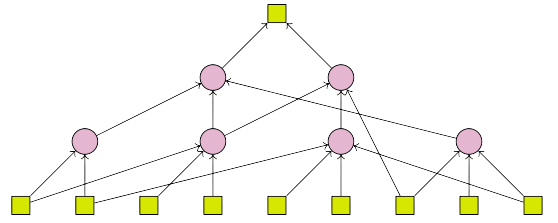
As we touched on before, a neural net is just many individual neurons stacked atop one another. More specifically, a given network is a horizontal stack of many layers, which are themselves vertical stacks of neurons. Computation happens as activations are propagated between adjacent layers, such that each neuron takes in all activations of the previous layer.

In other words, each entry in a given neuron's weight vector is multiplied with the activation of a neuron in the previous layer. So we can visualize each of these entries as a weighted edge connecting the current neuron to a neuron in the previous layer.

After computing the weighted sum these edges encode, adding a bias, and passing the whole thing through a non-linearity, we obtain a neuron's activation, which is propagated forward and becomes a part of the weighted sum computed by neurons in the next layer.

This view of the neuron, where we decompose each neuron's weight vector into a set of weighted edges, is admittedly slightly more messy and less elegant than our previous model. But as we don't know how to take the derivative with respect to an entire vector (yet), it is a necessary evil if we want to be able to optimize our parameters via gradient descent.

So how do we represent all this mathematically? Well, we can index each neuron by its layer and position in that layer. Each of a neuron's weights can then be indexed with one additional term, representing the position of the neuron it connects to in the previous layer. Thus, the activation of the \(i\)th neuron in the \(L\)th layer, given \(j\) neurons in the previous layer, is:

$$\alpha^{(L)}_i = \sigma\left(\sum\limits_{n=0}^j \alpha^{(L-1)}_n \cdot w^{(L)}_{(i, n)} + b^{(L)}_i\right)$$

If we were to repeatedly apply this expression, we would end up with a new expression representing the activation of the neuron in our network's final layer:

$$\sigma \left( \alpha^{(1)}_1 \cdot w^{(2)}_{(1,1)} + \alpha^{(1)}_{2} \cdot w^{(2)}_{(1,2)} + b^{(2)}_1 \right)$$

$$\bigg\downarrow$$

$$\sigma \left( \sigma \left( x^{(0)}_1 \cdot w^{(1)}_{(1,1)} + x^{(0)}_2 \cdot w^{(1)}_{(1,2)} + b^{(1)}_1 \right) \cdot w^{(2)}_{(1,1)} + \sigma \left( x^{(0)}_{1} \cdot w^{(1)}_{(1,1)} + \alpha^{(0)}_2 \cdot w^{(1)}_{(1,2)} + b^{(2)}_1 \right) \cdot w^{(2)}_{(1,2)} + b^{(2)}_1 \right)$$

And, unfortunately for us, it is this bulky expression we're going to have to pass into our error function, because it represents the network's prediction. Worse, we're going have to differentiate it with respect to each of our weights and biases to calculate the gradient.

But this expression is so convoluted, it's unclear where we would even start. Luckily, we can simplify things with a helpful model known as a computational graph, where the nodes of this graph represent some fundamental operations (e.g., addition, multiplication) and its edges represent the values flowing into these operations.

We think of each node as performing its operation on the values it receives, and then spitting out some output. What's more, by storing each node's output in some associated variable we can track all intermediate states an expression goes through before arriving at its final state – the last node in our graph – and this will turn out to be incredibly helpful.

Let's imagine constructing such a graph to represent the evaluation of our error function at this two-layer net's prediction for some labeled datapoint \((\boldsymbol{\vec{x}}, y)\). Calculating the gradient means finding the derivatives of the final node with respect to each of our weights and biases. To make things easier, we'll abstract away each node with some generic function.

With that in mind, let's examine the following segment of the graph. We see that we can represent our network's error as some composition of functions: \(\varphi = a(b(c(\xi, b^{(2)}_1)), y).\)

What we want is to find the derivative of this error with respect to the bias \(b^{(2)}_1.\) But because it is not a direct function of this bias, we must apply the chain rule.

The chain rule tells us that when trying to find the derivative of some expression with respect to a variable that it does not directly depend on, we must first find the derivative of that expression with respect to the variable it does directly depend on.

Each node in the graph directly depends on the node(s) before it, so, per the chain rule, we must calculate the derivative of each node with respect to its predecessor(s). Then we can construct another computational graph (known as the adjoint graph) that runs in the opposite direction, where each node passes down its derivative with respect to the previous node(s).

This might seem like a somewhat artificial construction, but bear with me for a minute – phrasing things in this way will make the solution to our problem just pop out. That said, now that we have identified all necessary derivatives, the chain rule tells us we must multiply them together to get our answer – the derivative of our error with respect to the bias.

And if we study the adjoint graph a bit more carefully, we see that all the derivatives we must multiply together \(\left(\frac{\partial \varphi}{\partial \tau}, \frac{d\tau}{d\pi}, \frac{\partial \pi}{\partial b^{(2)}_1}\right)\) lie somewhere on the path from \(\varphi\) to our bias \(b^{(2)}_1\). So we can compute the derivative in question simply by traversing the graph, accumulating all the derivatives being passed down from node to node, and multiplying them together.

And this fact is no less true for any other nodes in our graph. Since moving between any two nodes means encountering all the intermediary states between them, and as the chain rule is fundamentally a statement about how we must multiply the derivatives of these states when differentiating nested expressions, any path on this graph computes some derivative!

Moreover, we can imagine constructing such a graph for the whole network. Then calculating the gradient corresponds to traversing the paths from our final node to each weight and bias.

But we might notice that many of these paths are essentially the same, only diverging at the very end. For instance, consider the paths from \(\varphi\) to the weights \(w^{(1)}_{(1,1)}\) and \(w^{(1)}_{(1,2)}.\) They are equivalent except for two divisions – in other words, they differ by only two derivatives.

Traversing the graph two separate times – one for each weight – seems wasteful. Wouldn't it be better if we could somehow “remember” what the shared segment of their paths was, so we wouldn't have to re-traverse the whole graph all over again?

Then we could calculate the entire gradient in one traversal. To see this in action, imagine that every time we step to a new node we multiply the derivative the current node is passing down to it by all previous derivatives, and store it in some variable \(\delta_n\) denoting the local error signal – or the derivative of the error with respect to the current node.

Now, when we reach a branch in our graph – say where \(\pi\) branches out to \(\xi\) and the bias \(b^{(2)}_1\) – we have the derivative chain up to that point stored in the local error signal, so even if we choose to step to \(\xi\) first, we don't have to re-traverse the entire graph when we want to find the derivative with respect to the bias. We can just pick back up from where we left off.

This process of caching the current derivative chain in an associated variable for each node is called memoization and does wonders for our efficiency.

But the problem is not completely solved just yet. Even though we now know which derivatives we have to multiply together to find each element of the gradient, we still don't know what the actual numerical values for these derivatives are.

Calculating these values, however, is much easier than it might seem. Even though we've been dealing with each node as if it were some abstract function, in reality it's a rather simple operation – additions, multiplications, or applications of our non-linearity. And since we know the derivatives of these operations, finding the derivatives between nodes is trivial.

For instance, examine the node \(\iota\) in the graph above. It is the sum of two variables: the node \(\eta\) and the bias \(b^{(1)}_1\). So obviously the derivative with respect to both variables is just one.

We can similarly consider the node \(\epsilon\) which is the product of the first entry of our input vector \(x_1\) and the weight \(w^{(1)}_{(1,1)}\). Again, the derivative with respect to the weight is obviously \(x_1\).

It is worth noting that things aren't always this simple, though. The computational graph for a feedforward neural net is just some linear chain of nodes; there is only one path by which to reach each node. But as we up the complexity of our architectures with things like skip connections and recurrence, we can get graphs for which this property no longer holds.

That might seem like a problem at first – if there are multiple paths to a single node, then there are also multiple definitions for its derivative. So which one do we choose? The answer, perhaps unsurprisingly, is all of them, in that we add them all together.

This is just a more general version of the chain rule, what you might call the multivariable chain rule. If a variable depends on another variable in two different ways, then we have to sum up the derivatives of both of these dependencies in order to find the total derivative. In other words, the local error signal at a given node is the sum of all paths that lead to it.

$$\frac{d}{dx}(f(a(x), b(x))) = \frac{da}{dx}\frac{\partial f}{\partial a} + \frac{db}{dx}\frac{\partial f}{\partial b}$$

So what does all of this mean, taken together? Well, the first key idea here is that any complex expression we might want to differentiate – like our network's error – is actually just a composition of many elementary operations whose derivatives we already know. And a computational graph is nothing more than the visual manifestation of this composition.

Secondly, the chain rule provides us with a very straightforward way to find the derivatives of such compositions. And even though we, as humans, wouldn't usually use the chain rule, to, say, differentiate an expression like \(x^2 + 2x\), technically we could. After all, the chain rule is the only differentiation rule you really need to know – everything else follows from it. Plus, it generalizes rather nicely to the multivariable case – all we have to do is add paths together.

And this approach works great for computers, because it allows us to hardcode the expressions for only a few basic derivatives while still enabling them to differentiate pretty complex expressions. If we also think to memoize derivative chains, then what we get is an algorithm for quickly and efficiently computing exact derivatives, which is exactly what we need to make gradient descent viable.

An Algorithmic Perspective

Together, this entire process is known as reverse-mode automatic differentiation (AD). In the context of neural networks, though, it goes under another name: backpropagation.

But it's actually not the only way we could traverse a computational graph. After all, our decision to start at the end of the graph was an arbitrary one – we could have just as easily chosen to start at the beginning of the graph and propagate derivatives forward instead.

In fact, this method – forward-mode AD – and reverse-mode AD are conceptually equivalent, because they are just different ways of parsing the chain rule. Given some function composition \(f(g(h(x)))\), forward-mode computes derivatives from the inside-out, whereas reverse-mode does the opposite, computing them from the outside-in.

$$\left( \frac{dh}{dx} \right) \left( \frac{dg}{dh}\frac{dh}{df}\right) \hspace{2em} \text{vs.} \hspace{2em} \left( \frac{df}{dg}\frac{dg}{dh}\right) \left( \frac{dh}{dx} \right)$$

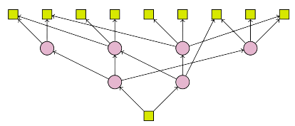
So why do we use reverse-mode in neural nets then? It has to do with the fact that each method is only optimal in a specific situation. For instance, let's imagine we want to differentiate some expression whose graph has many inputs but only a single output.

When using forward mode, we start at one of the input nodes and explore all the paths from that node to the output node. So after one pass through the graph, we end up with the derivative of the output with respect to that one input. Reverse-mode on the other hand – which explores the paths from the one output node to all input nodes – can get the derivatives of the output with respect to every input in a single go.

Of course, there's the flip side: when we have a graph with many outputs, but only a single input, forward-mode can grab everything in just a single run, since it only has to worry about one input anyway. In fact, we can use a special number system known as the dual numbers to make things run even faster. To get the same result using reverse-mode, we would have to traverse the graph multiple times.

The general rule is, given some function \(f : M \rightarrow N \), when \(M \gg N\) – when we have many more inputs than outputs – we should use reverse-mode, since forward mode will have to traverse the graph \(M\) times while reverse-mode will only have to traverse it \(N\) times. For the same reasons, when \(M \ll N\), forward-mode is the optimal method.

And obviously neural nets fit the first description – they are functions from millions or even billions of parameters (GPT-3, anyone?) to a single scalar loss (at least, during training). If we used forward mode to differentiate neural nets instead, our performance could potentially be millions of times worse!

Let's Vectorize!

But what we've described so far still isn't how things are done in practice. As I mentioned before, concerning ourselves with each individual each weight and bias is not the most efficient nor the most elegant way of doing things. Instead, a much cleaner conception of what's going on can be achieved by representing things in a vectorized fashion.

Given a \(k\)-neuron layer, with \(j\) neurons in the previous layer, we can stack the weights and biases of each of these neurons into a matrix and vector respectively.

$$\boldsymbol{W}^{(L)} = \begin{bmatrix} w^{(L)}_{(1, \hspace{0.1cm} 1)} & \cdots & w^{(L)}_{(1, \hspace{0.1cm} j)} \\ \vdots & \ddots & \vdots \\ w^{(L)}_{(k, \hspace{0.1cm} 1)} & \cdots & w^{(L)}_{(k, \hspace{0.1cm} j)} \\ \end{bmatrix} \in \mathbb{R}^{k \times j} \hspace{2cm} \boldsymbol{\vec{b}}^{(L)} = \begin{bmatrix} b^{(L)}_1 \\ b^{(L)}_2 \\ \vdots \\ b^{(L)}_k \\ \end{bmatrix} \in \mathbb{R}^{k}$$

Multiplying this matrix against the vector of previous activations yields a new vector containing the weighted sum each neuron computes. This is an equivalent construction to our earlier model, where each neuron dotted its weight vector against the incoming input vector, as matrix-vector multiplications are just a way of batching many dot products.

If we add this resulting vector to our bias vector and do an element-wise application of our non-linearity, then we have computed the vector of activations for that layer like so:

$$\boldsymbol{\vec{\alpha}^{(L)}} = \sigma\left(\boldsymbol{W}^{(L)}\boldsymbol{\vec{\alpha}}^{(L-1)} + \boldsymbol{\vec{b}}^{(L)}\right)$$

As before, our network's output is just some recursive composition of these layers, which we can also represent with a (noticeably more succinct) set of computational graphs.

The only problem here is that the derivatives being passed down in the adjoint graph are not scalar-to-scalar derivatives like we dealt with earlier, but vector-to-vector, or even vector-to-matrix derivatives. As such, we need to develop some reasonable notion of what these derivatives should look like.

Let's imagine some function mapping an input vector \(\boldsymbol{\vec{x}}\) to an output vector \(\boldsymbol{\vec{y}}.\) If we want to measure the effect varying the input vector has on the output vector (i.e., its derivative), we need to determine how each element of the input affects each element of the output.

In other words, we need to find the individual derivatives of each element of the output with respect to each element of the input, which we could organize into a matrix like so:

$$\begin{bmatrix} \frac{\partial{\boldsymbol{\vec{y}}_1}}{\partial\boldsymbol{\vec{x}}_1} & \cdots & \frac{\partial{\boldsymbol{\vec{y}}_1}}{\partial{\boldsymbol{\vec{x}}_n}} \\ \vdots & \ddots & \vdots \\ \frac{\partial{\boldsymbol{\vec{y}}_n}}{\partial{\boldsymbol{\vec{x}}_1}} & \cdots & \frac{\partial{\boldsymbol{\vec{y}}_n}}{\partial{\boldsymbol{\vec{x}}_n}} \\ \end{bmatrix}$$

In some sense then, this matrix is the derivative of that vector-to-vector function, because it represents all the ways the output vector could change given some infinitesimal nudge to the input vector. We refer to such a matrix as the Jacobian, and can think of it as a generalization of the gradient, since it similarly consolidates all of a function's derivative information.

In other words, each derivative being passed down in the adjoint graph is a Jacobian. So we can perform reverse-mode AD just like before, substituting matrix multiplication for the scalar kind. Of course, this requires storing the derivatives of some basic matrix operations: vector addition, matrix-vector multiplication, and element-wise function applications.

Let's start out easy with vector addition. Remember, calculating the Jacobian means differentiating each entry of the output with respect to each entry of the input.

$$\frac{\partial}{\partial{\boldsymbol{\vec{x}}}}\left( \begin{bmatrix} x_1 \\ x_2 \\ \vdots \\ x_n \\ \end{bmatrix} + \begin{bmatrix} y_1 \\ y_2 \\ \vdots \\ y_n \\ \end{bmatrix}\right) = \begin{bmatrix} \frac{\partial}{\partial{x_1}}(x_1 + y_1) & \cdots & \frac{\partial}{\partial{x_n}}(x_1 + y_1) \\ \vdots & \ddots & \vdots \\ \frac{\partial}{\partial{x_1}}(x_n + y_n) & \cdots & \frac{\partial}{\partial{x_n}}(x_n + y_n) \\ \end{bmatrix}$$

In this case, the result is the identity matrix \(\boldsymbol{I}.\) This offers a nice parallel to classical calculus, as differentiating the sum of two different variables also returns the multiplicative identity.⁵

Slightly more complex is the idea of differentiating a matrix-vector product with respect to the vector. It turns out though that this also has a nice interpretation under the rules of classical calculus, if we think of the matrix as a coefficient. Setting up the Jacobian:

$$\frac{\partial}{\partial{\boldsymbol{\vec{x}}}} \left( \begin{bmatrix} a & b \\ c & d \end{bmatrix} \begin{bmatrix} x_1 \\ x_ 2 \\ \end{bmatrix} \right) = \begin{bmatrix} \frac{\partial}{\partial{x_1}}(ax_1 + bx_2) & \frac{\partial}{\partial{x_2}}(ax_1 + bx_2) \\ \frac{\partial}{\partial{x_1}}(cx_1 + dx_2) & \frac{\partial}{\partial{x_2}}(cx_1 + dx_2) \\ \end{bmatrix}$$

We see that it simplifies to the matrix \(\boldsymbol{W}.\) In other words, the derivative of a matrix-vector product with respect to the vector is the matrix the vector is being multiplied by.

But what if we want to differentiate this product the other way around, with respect to the matrix? This is a bit harder, because differentiating each entry of a vector with respect to each entry of a matrix means we'll need multiple matrices, one per element of our output.

The generalization of a matrix to higher dimensions is known as a tensor, and they're not the most pleasant things to work with. But if we examine the situation more closely, we'll see that it is actually possible to represent the Jacobian in matrix form. To see what I mean, let's try differentiating only a single element of the output vector \(\boldsymbol{\vec{y}}\) with respect to the matrix.

$$\frac{\partial{\boldsymbol{\vec{y}}}_1}{\partial{\boldsymbol{W}}} = \begin{bmatrix} \frac{\partial}{\partial{a}}(ax_1 + bx_2) & \frac{\partial}{\partial{b}}(ax_1 + bx_2) \\ \frac{\partial}{\partial{c}}(ax_1 + bx_2) & \frac{\partial}{\partial{d}}(ax_1 + bx_2) \\ \end{bmatrix}$$

Simplifying, we see that the resulting matrix only has one non-zero row. Furthermore, we would find that this trend holds for any matrix-vector product we could imagine. And if we think about it, this makes sense, too – after all, each element of the output vector only depends on one row of the actual matrix, so all its other derivatives will be zero.

If we do this for each element in our output vector, then we get a series of mostly non-zero matrices with only a single row filled in. But the filled-in rows for each of these matrices never collide, because each element of the output vector depends on a different row of the matrix.

$$\frac{\partial{\boldsymbol{\vec{y}}}_1}{\partial{\boldsymbol{W}}} = \begin{bmatrix} x_1 & x_2 \\ 0 & 0 \\ \end{bmatrix} \hspace{1cm} \frac{\partial{\boldsymbol{\vec{y}}}_2}{\partial{\boldsymbol{W}}} = \begin{bmatrix} 0 & 0 \\ x_1 & x_2 \\ \end{bmatrix}$$

So even though the Jacobian, as we've previously defined it, should be some 3D stack of these matrices – some tensor – because none of their non-trivial entries interfere, we could imagine smushing this 3D stack down into a single matrix. Thus:

$$\frac{\partial}{\partial{\boldsymbol{W}}} \left( \begin{bmatrix} a & b \\ c & d \end{bmatrix} \begin{bmatrix} x_1 \\ x_ 2 \\ \end{bmatrix} \right) = \begin{bmatrix} x_1 & x_2 \\ x_1 & x_2\\ \end{bmatrix}$$

The final derivative we must consider is that of element-wise function applications – such as with our non-linearity – where an element-wise function is defined like so:

$$f\left( \begin{bmatrix} x_1 \\ x_2 \\ \vdots \\ x_n \\ \end{bmatrix} \right) = \begin{bmatrix} f(x_1) \\ f(x_2) \\ \vdots \\ f(x_n) \\ \end{bmatrix}$$

The Jacobian of such a function, then, looks something like this, where the diagonal entries hold the derivative of the function, and all non-diagonal entries are zero:

$$\begin{bmatrix} \frac{\partial}{\partial{x_1}}(f(x_1)) & \cdots & \frac{\partial}{\partial{x_1}}(f(x_n)) \\ \vdots & \ddots & \vdots \\ \frac{\partial}{\partial{x_1}}(f(x_n)) & \cdots & \frac{\partial}{\partial{x_n}}(f(x_n)) \\ \end{bmatrix} = \begin{bmatrix} f\prime & 0 & \cdots & 0 \\ 0 & f\prime & \dots & 0 \\ \vdots & \vdots & \ddots & \vdots \\ 0 & 0 & \cdots & f\prime \end{bmatrix}$$

Moreover, matrix multiplying against a diagonal matrix like this one is analogous to performing element-wise multiplication against a matrix filled with whatever is occupying this diagonal,⁶ where the element-wise – or Hadamard – product is denoted \(\boldsymbol{A} \odot\boldsymbol{B}.\) This is what we tend do in practice, because it is much more efficient than matrix multiplication.

In fact, the whole reason we vectorize to begin with is because bundling things into matrices and doing batch operations is faster than doing things one-by-one. And knowing only these matrix calculus primitives, we can pretty much differentiate through any vanilla neural net!

The Generalized Chain Rule

I would be remiss if I didn't mention one more thing though. Isn't it kind of convenient how the chain rule just automatically generalized to Jacobians? Why did that happen?

It has to do with the deeper definition of derivatives as linear maps. Even if we don't often think of them in this way, derivatives naturally satisfy the two properties of linearity: the derivative of a sum is the sum of derivatives, and the derivative of a function times a scalar is the derivative of that function times the scalar (English kind of breaks down here...).

$$D(f + g) = Df + Dg \hspace{1cm} D(cf) = c(Df)$$

In other words, we're always working with Jacobians, where a Jacobian represents all the ways a function could change given some nudge to its input. And the chain rule is nothing more than a statement about the Jacobian of a function composition, which says that given two functions \(f\) and \(g\), the Jacobian of their composition \(f(g(x))\), where \(x\) could be a scalar, vector, matrix, or even tensor, is the Jacobian of \(f\) at \(g\) composed with the Jacobian of \(g\) at \(x\).

$$D(f \circ g)(x) = Df(g(x)) \circ Dg(x)$$

So it's not that the chain rule magically generalizes to Jacobians – it's defined in terms of them to begin with. Traditional, single-variable calculus just doesn't expose them in their full generality. And the only reason there's a notion of multiplication in the chain rule in the first place is because composing linear maps is defined as matrix multiplication.

That's is a long-winded way of saying that the derivative is the Jacobian - they're equivalent concepts. And the different branches of calculus just study increasingly less specialized versions of it. In that sense, all automatic differentiation does is compute a Jacobian-vector product, or the Jacobian at a specific input.

Thinking about things in terms of Jacobians also highlights an important difference between forward-mode and reverse-mode. As we acknowledged before, one pass with forward-mode computes the derivatives of all outputs with respect to a single input, while one pass with reverse-mode computes the derivatives of a single output with respect to all inputs.

$$\begin{bmatrix}\frac{\partial{\boldsymbol{\vec{y}}}_1}{\partial{\boldsymbol{\vec{x}}}_1} \\ \frac{\partial{\boldsymbol{\vec{y}}}_2}{\partial{\boldsymbol{\vec{x}}}_1} \\ \vdots \\ \frac{\partial{\boldsymbol{\vec{y}}}_n}{\partial{\boldsymbol{\vec{x}}}_1} \\ \end{bmatrix} \hspace{1cm}\textrm{vs.} \hspace{1cm}\begin{bmatrix}\frac{\partial{\boldsymbol{\vec{y}}}_1}{\partial{\boldsymbol{\vec{x}}}_1} & \frac{\partial{\boldsymbol{\vec{y}}}_1}{\partial{\boldsymbol{\vec{x}}}_2} & \ldots & \frac{\partial{\boldsymbol{\vec{y}}}_1}{\partial{\boldsymbol{\vec{x}}}_n} \end{bmatrix}$$

In other words, forward-mode computes the Jacobian column-by-column whereas reverse-mode does so row-by-row. That's why functions with many outputs (many rows) are better suited to forward-mode and those with many inputs (many columns) to reverse-mode.

Differentiable Programming

That's pretty much a wrap, but there's one more essential idea about AD worth mentioning: it's not just limited to typical mathematical expressions. Anything that can be represented as a computational graph is fair game. That includes control flow constructs like loops and conditionals, and so as a consequence, entire programs can be differentiated over too!

This is where the idea of differentiable programming was borne: automatic differentiation that can run directly on programs. We're still a ways off from being able to do this (the extent of our differentiable programs right now – neural nets – are basically just increasingly inventive compositions of matrix multiplication), but this is where things are headed in the future, and personally, I think a good language for differentible programming will take the whole deep learning paradigm to the next level.

All that is for another time, but the main thing to take away from this is that as a tool, automatic differentiation is very flexible, and can give us some notion of a derivative even where classical calculus fails. Differentiable programming seems like an especially promising application of this flexibility, but it is certainly not the only one.

Conclusion

So to recap, automatic differentiation is a way of quickly computing derivatives with computers. It has both a forward-mode and reverse-mode implementation, the latter of which is used in neural nets. And like all truly great ideas it is based on a simple, but piercing insight: that the amount of expressions we can differentiate grows exponentially with the amount of elementary derivatives that we know. In other words, the chain rule is a lot more powerful than we may always give it credit for.

It also shows us the power in simple tricks such as a memoization – tools of the trade from a branch of computer science known as dynamic programming. Even if something looks like it'd be expensive to compute at first glance, it might be unintuitively cheap once we figure out how to reuse computation and reduce redundancy.

All in all, automatic differentiation is one powerhouse of an algorithm, often cited as one of the most important ones to have come forward in the twentieth century. Understanding it well opens up many doors in scientific computing and beyond, and the field is still being actively researched. Given that neural networks only discovered it relatively recently,⁷ it might very well be that there are other killer applications of the technique yet to be found. After all, there's not much you can't solve with derivatives.

Acknowledgements

Thank you to Dr. John McKay for taking the time to proofread this post.

Resources

• Håvard Berland's Slides
• Calculus on Computational Graphs
• How to Differentiate with a Computer
• Computing Neural Network Gradients
• Vector, Matrix, and Tensor Derivatives
• Automatic Differentiation in Machine Learning: A Survey
• The CS 6120 Course Blog: Automatic Differentiation in Bril

Footnotes

1. It's relatively trivial to demonstrate this:

$$\begin{aligned} \lim_{h\to 0} \frac{f(x+h, y) - f(x, y)}{h}\hspace{1cm} &\textrm{(Definition of the derivative of } f(x,y) = x^2 + y^2 \hspace{0.1cm}\textrm{ w.r.t to } x) \\ \\ \lim_{h\to 0} \frac{(x+h)^2 + y^2 - (x^2 + y^2)}{h}\hspace{1cm} &\textrm{(Simplification)} \\ \\ \lim_{h\to 0} \frac{(x+h)^2 - x^2}{h}\hspace{1cm} &\textrm{(Definition of the derivative of } f(x) = x^2 \hspace{0.1cm}\textrm{ w.r.t to } x) \end{aligned}$$

As you see, \(y\) washes out. Another way to think about this is that since \(y\) isn't being nudged by some infinitesimal \(h\) like \(x\) is, its presence in the first term will be completely canceled out by its presence in the second, which is just another way of saying that since it isn't changing, it is invisible as far as the derivative is concerned. ↩

2. The simplest error function you could have is just the difference between the prediction and the label: \(E(\hat{y}, y) = \hat{y} - y.\) In practice we actually square this difference to accentuate really bad predictions and so that we don't have to deal with a negative result. This is known as the square error: \(E(\hat{y}, y) = (\hat{y} - y)^2.\) ↩

3. What is \(\theta\) doing in the subscript of the gradient symbol? It's just a way of saying that even though our function also takes in an input and a label, we don't want to include their partials in our gradient – after all, we can't change our input or label, those two pieces of information are set for the problem. ↩

4. \(\eta\) is a hyperparameter, or a variable the neural net does not learn by itself, but must be explicitly set. It's known as the learning rate, since it controls how quickly we descend the error-surface, and thus how fast we learn. ↩

5. All this means is that addition is some operation, that, when you change its inputs, reflects the exact same change in its output, whether these inputs be vectors, or scalars. ↩

6. A demonstration of this property with concrete matrices:

$$\begin{align} \begin{bmatrix} a & b \\ c & d \\ \end{bmatrix} \begin{bmatrix} x & 0 \\ 0 & x \\ \end{bmatrix} = \begin{bmatrix} ax & bx \\ cx & dx \\ \end{bmatrix}\hspace{1cm}&\textrm{(Multiplication against diagonal matrix)} \\ \\ \begin{bmatrix} a & b \\ c & d \\ \end{bmatrix} \odot \begin{bmatrix} x & x \\ x & x \\ \end{bmatrix} = \begin{bmatrix} ax & bx \\ cx & dx \\ \end{bmatrix}\hspace{1cm}&\textrm{(Hadamard product)} \end{align}$$

As you can see, they are equivalent. But whereas the Hadamard product only has to do \(N \times M\) operations when multiplying two \(N \times M\) matrices, matrix multiplication has to do \(N \times M \times M \times (M - 1)\) operations. ↩

7. While researching for this post, I found out that before AD was commonly used, neural net researchers would analytically calculate the derivatives for their networks by hand and then hardcode them into computers. So obviously networks couldn't be deep! Read more here! ↩