The transformer – a neural net architecture proposed in Vaswani et al., 2017 – has taken the NLP world by storm in the past few years, contributing to the recent success of OpenAI's GPT-3 among many others. But while there is an abundance of online material describing the transformer architecture, its crucial theoretical contribution – the key, query, and value attention mechanism – lacks a clear, accessible explanation, especially from the perspective of what motivated it and why it works. The focus of this post is to hopefully provide some of that intuition, and demonstrate why the attention mechanism is so powerful.

Attending To Thy-Self

Before we delve further into how the transformer phrases self-attention mathematically, it's worth clarifying what exactly “self-attention” means. Just like a standard layer of neurons, the self-attention operation is some parameterized, differentiable function we can include in our neural nets. Unlike these layers though, it works on sets of vectors (rather than vectors themselves), and learns some function to linearly combine each element with all the others.

You can think of it a bit like a blender: it blends all other elements into the current element, creating some new hybrid element that contains contextual information about the set as a whole. The intuition here is that the network is learning to focus some of its “attention” on elements other than the one it is currently processing, hence the operation's name.

And this turns out to be incredibly helpful, especially in situations where context matters (like understanding language). What's more, it offers a distinctive advantage over other, more traditional ways of embedding context, like recurrent neural nets.

RNNs try and smush the whole context into a single vector. This compression means that some information will inevitably be lost, especially as the text being interpreted gets longer and more complex. Moreover, only a small part of this vector may actually be useful to any given element, and having to block out the noise introduces unnecessary complexity.

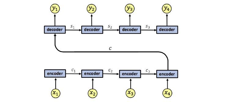
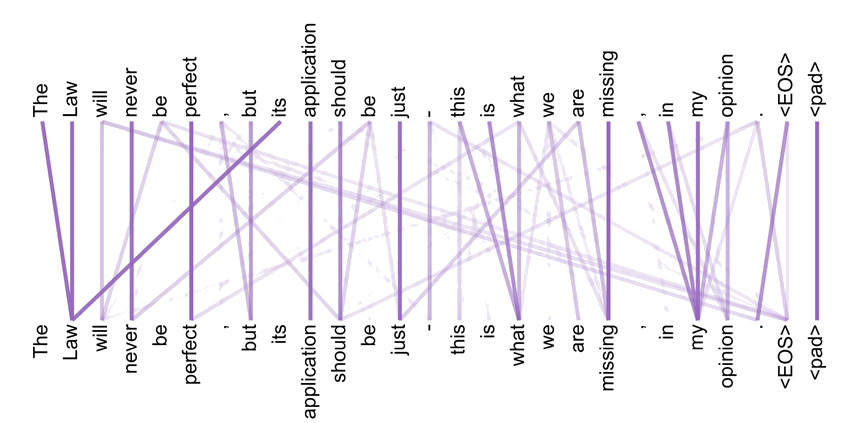
Self-attention, on the other hand, allows any element of the input to directly attend to any other element. As such, each element gets to define its own unique context vector! And since it only has to account for the local context (unlike in RNNs), this vector can be much more precise about the information it does contain.

But how exactly does a given element decide how much to attend to another element? And how does it use this information to build up its associated context vector? To get to the real meat of the attention mechanism, we need to start phrasing things mathematically.

Let's imagine we have a matrix \(\boldsymbol{V}\) that contains the vector representations of some input text in its columns. Suppose we also have a vector \(\boldsymbol{\vec{\alpha}}\) which contains the attention coefficients for one of these words (i.e., how much that word wants to attend to every other word).

$$\boldsymbol{V} = \begin{bmatrix} \vert & \vert & \hspace{1cm} & \vert \\ \boldsymbol{\vec{v}_1} & \boldsymbol{\vec{v}_2} & \cdots & \boldsymbol{\vec{v}_n} \\ \vert & \vert & \hspace{1cm} & \vert \\ \end{bmatrix} \in \mathbb{R}^{n \times m} \hspace{2cm} \begin{align} \boldsymbol{\vec{\alpha}} &= \begin{bmatrix} \alpha_{1} \\ \alpha_{2} \\ \vdots \\ \alpha_{n} \\ \end{bmatrix} \in \mathbb{R}^{n} \end{align}$$

When computing the new representation for this word, we want it to incorporate other words such that it more strongly incorporates words with which it has a high attention coefficient, and more weakly incorporates those with which it has low attention coefficient.

The easiest way to do this is by a weighted sum (of vectors), \(\alpha_1 \boldsymbol{\vec{v}_1} + \alpha_2 \boldsymbol{\vec{v}_2} + \ldots + \alpha_n \boldsymbol{\vec{v}_n}.\) This is equivalent to the matrix-vector product \(\boldsymbol{V}\boldsymbol{\vec{\alpha}}.\) In other words, calculating this matrix-vector product gives us our chosen word's specific context vector.

However, we still need to find some function that is capable of computing the vector \(\boldsymbol{\vec{\alpha}}\) for each word in the first place. Given the embeddings of two words, it needs to determine how strongly one should attend to the other (and vice versa).

Intuitively, it makes sense that the more similar two words are, the more they would want to attend to one another. So perhaps we can just define the attention coefficient between two words as the dot product of their embeddings.

Unfortunately, this idea has two key flaws that stop it from working outright. To see what I mean, consider the words “hot” and “cold”. For now, we're going to make the simplification that word-embeddings only reflect word-meaning. In other words, the representations for “hot” and “cold” should point in opposite directions, since they are antonyms.

However, it's also likely that both words will want to attend highly to the word “temperature”, as in the phrase “The temperature is hot” or “The temperature is cold”. If both “hot” and “cold” want to attend highly to “temperature”, then their embeddings must be close to its embedding, as that's the only way they will yield a high dot product with one another, and thus – as we've defined it – a high attention coefficient.

But by making the representations of “hot” and “cold” closer to the representation of “temperature”, we are necessarily making them closer to one another, and therefore losing the information that they are antonyms!

In other words, it's not possible to encode data about attentional relationships into our word-embeddings without compromising the information about semantic relationships that's already there. Dot production attention requires that we choose between one or the other.

Of course, it's worth noting that this argument is extremely low-dimensional. In the thousand-dimensional vector spaces that our word-embeddings actually occupy in practice, there are several more degrees of freedom for the neural network to play around with. However, at the very least, it is easy to recognize that these two different pieces of information can lead to competing effects, and that there may be a better way to store them.

As if that wasn't bad enough, there's another, arguably even worse problem. Attention is not a mutually reciprocal action, but similarity is.

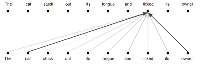
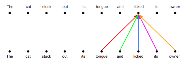
Consider the sentence “He picked up the tennis ball and found it was wet.” We would probably expect “it” to attend highly to “ball” (what “it” is referring to) while “ball” would probably attend highly to “tennis” and “picked up” (its type and the action performed on it), but much more weakly to “it” (after all, what new information does it gain from this?).

However, even though it might be more advantageous for “ball” to attend weakly to “it”, so long as “it” attends strongly to “ball”, “ball” must attend to “it” with equal strength.¹ This is because making “it” closer to “ball” necessarily makes “ball” closer to “it” by an equal amount.

More generally if a word X attends highly to another word Y, then Y must attend as highly to X by default. Furthermore, since X is similar to Y it is also similar to those words which are also similar to Y (words which Y attends highly to) and by extension those words which are similar to those words which are similar to Y (the words the words similar to Y attend highly to) and so on and so forth. Thus, everything will end up attending to everything else!

Evidently, using similarity as a metric for self-attention comes with its problems. But if we could get it to work, a dot product attention mechanism would be awfully nice. And it seems to make a great deal of intuitive sense as well. So how can we resolve its shortcomings?

Keys, Queries, and Values

The answer, in fact, is deceptively simple: with multiple embedding spaces. Let's consider our first problem again. There wasn't enough room in a single word-embedding to hold information about both word meaning and attentional relationships.

The natural thing to do, then, would be to distribute this information throughout multiple representations, as opposed to trying to cram it all into just one.

So let's create two embedding spaces. In \(\boldsymbol{E_1}\), the vector representation of each word will encode the semantic information associated with that word. It is in this space that “hot” and “cold” will be oppositely positioned. Conversely, in \(\boldsymbol{E_2}\), word-embeddings will hold attentional information – here, “hot” and “cold” will be close together along with “temperature”. But this is no longer an issue, as we have preserved the information that they are antonyms within \(\boldsymbol{E_1}\)!

This seems to solve our first problem, but it doesn't do much to help us with our second one. By having “hot” and “cold” attend highly to “temperature”, we're still forcing it to attend highly to them, as well (which it may actually want to do, but shouldn't have to).

Luckily for us though, this has a very similar fix: add another embedding space. More specifically, we need to split our second embedding space, \(\boldsymbol{E_2}\), into two separate spaces.

Let's call them \(\boldsymbol{E_q}\) and \(\boldsymbol{E_k}.\) We can then define self-attention as follows. When calculating self-attention with respect to “it” (i.e., how much “it” attends to “ball”) we dot its embedding in \(\boldsymbol{E_q}\) with the embedding of “ball” in \(\boldsymbol{E_k}.\) Likewise, dotting the representation of “ball” in \(\boldsymbol{E_q}\) with that of “it” in \(\boldsymbol{E_k}\) will give us self-attention with respect to “ball”.

As both operations deal with different embeddings (“it” in \(\boldsymbol{E_q}\) and “ball” in \(\boldsymbol{E_k}\) vs. “ball” in \(\boldsymbol{E_q}\) and “it” in \(\boldsymbol{E_k}\)) attention doesn't reciprocate. But, what is the intuition behind this operation?

Essentially, what we're doing is computing two representations for each word: one is a “key”, and the other is a “lock”. Computing self-attention with respect to some word X is a matter of seeing how similar other words' lock-representations are to its key-representation.

But just because a word Y's lock-representation is similar to X's key-representation doesn't imply the opposite – its key-representation may not be similar to X's lock representation!

To adopt the transformer's lingo, we refer to these key- and lock-representations as queries (key-representations) and keys (lock-representations), respectively. Put simply, a word's key is the information it chooses to expose about itself (the lock), while its query is the information it looks for in other words, when determining how much to attend to them (the key).

For example, the query of the word “it” might be something like “I attend highly to nouns – are you a noun?”, while its key might be “I am a pronoun”. Since the key of “ball” is “I am a noun”, it would strongly satisfy the query of “it”, causing “it” to attend highly to “ball”.

But crucially, since the key of “it” doesn't answer the query of “ball” with similar strength (“I attend highly to adjectives – are you an adjective?”), “ball” will attend very weakly to “it”.

We can visualize this idea even more viscerally by overlaying the embedding spaces containing our keys and queries atop one another. When doing so, we see that the angle formed between the key of “it” and the query of “ball” is different from the angle formed between the key of “ball” and the query of “it”. Different angles means different dot products means different attention coefficients!

So what's the mathematics behind all of this, then? How do we formalize these ideas? Let's imagine that we are given some sentence of variable length and need to find \(\boldsymbol{\vec{\alpha}}\) for the \(i\)th word in this sentence. Given this word's query \(\boldsymbol{\vec{q}}\) and the matrix \(\boldsymbol{K}\) whose columns are the keys of each word in the input, we can calculate it like so:

$$\boldsymbol{\vec{\alpha}} = \boldsymbol{K}^\top\boldsymbol{\vec{q}}$$

This is equivalent to dotting \(\boldsymbol{\vec{q}}\) with each entry of \(\boldsymbol{K}\) and storing the results in a vector, which is exactly how we defined key-query attention. But calculating \(\boldsymbol{\vec{\alpha}}\) isn't our true goal. What we really want to compute is \(\boldsymbol{\vec{\gamma}},\) our current word's context vector. And, as we realized earlier, this is just the product of \(\boldsymbol{\vec{\alpha}}\) with the matrix containing the semantic representations of all words.

We had said that these representations lived in the embedding space \(\boldsymbol{E_1}\), but to be consistent with the transformer's jargon, we'll rename it to \(\boldsymbol{E_v}\). Just as key- and lock-representations became queries and keys, we will refer to a word's semantic representation as its value.

In this vocabulary, self-attention is a sum of words' values weighted by their attention coefficients, or the dot product of their key with the current word's query. Thus:

$$\boldsymbol{\vec{\gamma}} = \boldsymbol{V}\boldsymbol{K}^\top\boldsymbol{\vec{q}} \hspace{1cm}$$

Sprouting Multiple Heads

Given all the complexities we encountered, it's surprisingly satisfying to see everything reduce to such a simple formula! But there's one glaring detail that we've glossed over so far. We've been assuming that our initial representation for each word is its semantic representation, or value. So where do its key and query come from?

Instead of first working with our word's value, we might imagine starting with some more general, abstract representation, that has a broad idea of word meaning, grammar, syntax, etc., but nothing too specific. We can then learn a series of weight matrices to linearly project this representation in three different ways, yielding the word's query, key, and value.

$$\boldsymbol{Q} = \boldsymbol{X}\boldsymbol{W_Q} \hspace{1cm} \boldsymbol{K} = \boldsymbol{X}\boldsymbol{W_K} \hspace{1cm} \boldsymbol{V} = \boldsymbol{X}\boldsymbol{W_V} $$

The query weight matrix might, for example, pull out the specific parts of this representation that store the types of words our word is usually accompanied by, while the key weight matrix might project it into a space that is more aware of grammar, tense, and part-of-speech. Of course, the attention mechanism is much more complex than this, and still not entirely understood, but rationalizing it in this way helps us understand why it works so well.

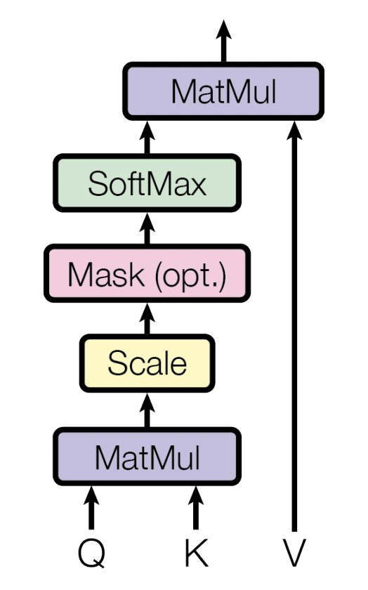
Moreover, adopting this perspective also allows us to rewrite our self-attention equation to operate on an entire matrix of word-embeddings. If we also sprinkle in a softmax and dimensionality constant to keep numbers from getting to large, we get:²

$$\textrm{Attention}(\boldsymbol{Q}, \boldsymbol{K}, \boldsymbol{V}) = \textrm{softmax}\left( \frac{\boldsymbol{Q} \boldsymbol{K}^T}{\sqrt{d_k}} \right)\boldsymbol{V}^T$$

The full picture, then, is as follows. The self-attention mechanism is parameterized by three learned weight matrices, each of which projects our general word representation into a specific space, which themselves each prioritize a different aspect of the word's identity. By multiplying together a word's representations in these three spaces we can produce its new representation, or context vector.

It's also worth considering how self-attention matches up with the convolution operation. They have some striking similarities. Both are fundamentally ways of embedding context. The key difference between the two is that attention has no limiting receptive field. It can model arbitrarily long-distance interactions, while convolutions operate on a predetermined scale.

This makes attention seem like the clear winner. But there is also a less obvious advantage to convolutions that doesn't become clear until we try to express attention as a convolutional kernel itself. For example, the attention kernel for a single word would look like this:

$$\boldsymbol{A} = \begin{bmatrix} \alpha_1 & \alpha_2 & \hspace{1cm} & \alpha_n \\ \vdots & \vdots & \cdots & \vdots \\ \alpha_1 & \alpha_2 & \hspace{1cm} & \alpha_n \\ \end{bmatrix} \in \mathbb{R}^{n \times m}$$

Seen in this way, it is intuitively obvious that an attention kernel is less expressive than an arbitrary convolutional one. Attention is a convolutional kernel where the values are the same in all columns. In particular, they are the attention coefficients of the word in question with respect to the word represented by that column. That's because attention is simply a weighted sum. It is just mixing together what already exists in different proportions.

Convolutions, on the other hand, have no such limitation. They can transform the input in a much more complex way than a weighted sum. In fact, they actually do several linear transformations based on the relative position of each of the elements in the input.

This reveals a drawback of our current attention mechanism. While the weighted sum operation it is doing makes intuitive sense, it also limits the types of new representations we can create, confining us to the subspace spanned by the specific words in the input.

We can think of this problem in another way, too. Even though our idea of creating context vectors for each word was a good first step, we need to go even further. Our key-query attention scheme is overworked. It's trying to consider all of the meanings and relationships of each word with respect to the current word, and then condense this information into a single representation, all in one go. Once again, we are straining our information capacity.

We might instead imagine using multiple such attention mechanisms, where each attention mechanism focuses on a specific aspect of each word. For example, instead of relying on one attention mechanism to recognize that a verb should attend highly to both the person doing it and the object it's being done to, we could split up this work between two separate attention mechanisms. In this way, each attention mechanism can specialize, and develop its own niche.

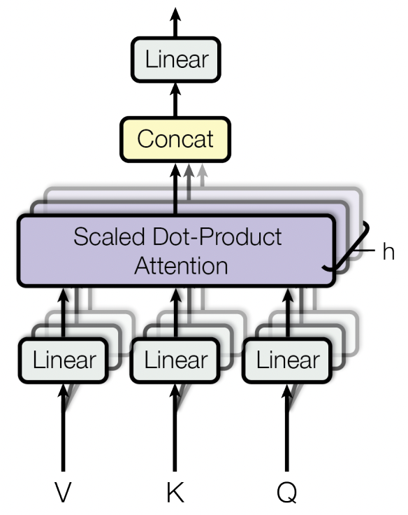
Mathematically, this means that instead of learning one set of three projection matrices, we will learn multiple such sets – one for each attention mechanism, which we'll call attention heads. If we then compute the relevant keys, queries, and values and plug them into the attention formula, we end up with multiple context vectors for each word, one per attention head.

Now we're left with the task of combining this set of context vectors into a single context vector for each word. There is a lot of potential choice for how to do this, but the transformer paper chooses to concatenate³ the output of each attention head, resulting in a matrix containing that head's recommendation for what each word's context vector should be. This matrix is then multiplied by one final projection matrix. So the formula for multi-head attention is:

$$\begin{aligned} \textrm{MultiHead}(\boldsymbol{Q}, \boldsymbol{K}, \boldsymbol{V}) &= \textrm{Concat}(\textrm{head}_1, \ldots, \textrm{head}_h)\boldsymbol{W^O} \\ \textrm{where head}_i &= \textrm{Attention}\left( \boldsymbol{X}\boldsymbol{W_Q^i}, \boldsymbol{X}\boldsymbol{W_K^i}, \boldsymbol{X}\boldsymbol{W_V^i} \right) \end{aligned}$$

It's worth noting that the argument we used to motivate multi-head attention is still pretty hand-wavy, and how useful having multiple heads really is is still an issue up for debate. Many papers have found that ablating (or getting rid of) a vast majority of the attention heads in a transformer can actually have minimal effects on performance. However, it seems that – for now at least – the conventional knowledge still mostly holds: two heads are better than one.

Conclusion

There you have it: an intuitive, visual understanding of the attention mechanism! Really, it's all about grappling with some of the intrinsic properties of vectors, and providing the underlying neural net with ample opportunity to spread information out across multiple sources before pooling it all together. This design seems simple in hindsight, but therein lies the engineering genius of the transformer architecture.

Even so, we've still just dipped our toes into the idea of attention. For one, the parallel between attention and convolutions given above was highly simplified, and there is a growing body of research (see this paper for an example) trying to better understand this relationship, especially as attention makes inroads into the field of computer vision.

Other efforts have tried to model attention from a mechanistic, circuit-level point of view, and have also seen some pretty interesting results as of late. Even more recently, attention has been linked to ideas such as Hopfield Networks and, as a result, spin systems.

That's to say that many of these ideas are still very much in flux. And now that we've laid the groundwork for understanding the what, why, and how of the attention mechanism, I'm itching to explore them in all of their glory in future blog posts! So stay tuned for more!

Acknowledgements

Thank you to Dr. Aidan Gomez – a co-author of the original transformer paper – for taking the time to read my first draft of this post, and for his words of encouragement. A very special thanks also to Llion Jones (another transformer co-author!) who provided both exciting conversation and invaluable feedback, especially in regards to maintaining technical correctness with my intuitive arguments.

Resources

• Attention Is All You Need
• Ashish Vaswani's 2019 Lecture
• Yannic Kilcher's Video on the Transformer

Footnotes

1. This leads to a certain Newton's Third Law of Attention: each act of attention induces an equal and opposite act of attention. Of course, we don't want this property! ↩

2. Actually, this equation isn't perfectly identical to what appears in the transformer paper. That's because we chose to put our word-embeddings in the columns of each matrix (as opposed to the rows, which is what the paper does) for ease of visualization, and so had to add in a few transposes. ↩

3. In talking with Llion Jones, I learned that the first version of the transformer actually added the outputs of the heads together instead of concatenating them. However, since then concatenation has become the de facto standard, so we will proceed with this choice. ↩